

This is another one of my articles about Microsoft Excel covering conditional formatting and conditional statement functions such as TRUE, FALSE, NOT, IF, AND, OR, XOR, IFNA and IFERROR.
Conditional formatting allows you to display your workbook cells differently based on specified criteria (the values of cells). Conditional functions allow you to present results in your cells based on different criteria. So one is for the display conditions and the other for the values returned based on a conditional statement.
Conditional formatting
We will start with conditional formatting and with a very simple example. I have a spreadsheet with some (fictional) purchases I made a few years back. Column A shows the name of the purchase, Column B shows the price I paid and Column C shows the current value if I were to sell it today. I’ve used Column D to calculate the profit or loss “=Present_Value-Original_Value” and Column E to show that as a percentage “=ROUND(Difference/Original_Value,2)“.
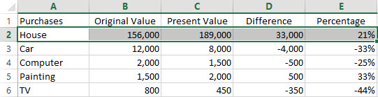
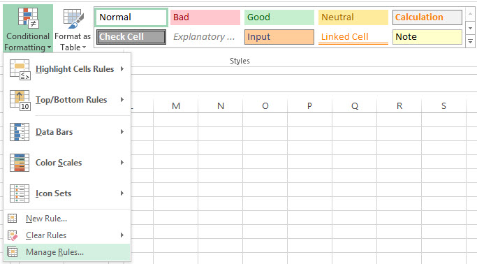
Now what I want to do is show the row background colour in green if I am in profit or orange if I have made a loss. First I want to set the conditional formatting for the first row so I’ve selected A2 to E2. Then on the Home tab, I have selected Conditional Formatting, Manage Rules. I could have selected New Rule but as my default background is not green or orange I will need to add two rules.
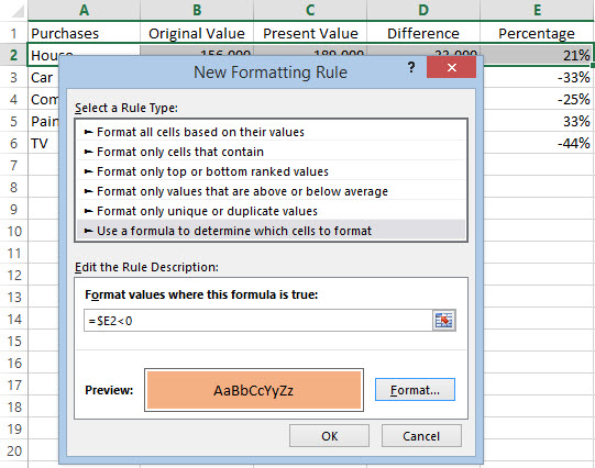
From the Conditional Formatting Rules Manager add a New Rule. Then select Use a formula to determine which cells to format. As we are on row 2, our formula will apply to this row. Enter =$E2<0 in the Format values where this formula is true box and select a background colour of orange by using the Format button. If you have selected the cell from the sheet remember to alter it so the $ symbol is only before the column indicator E.
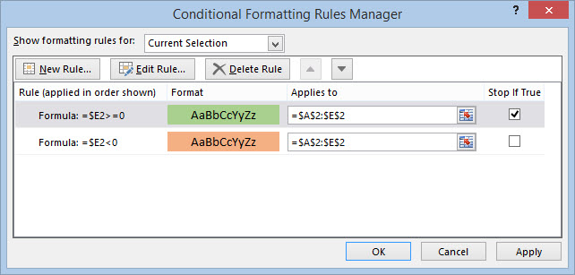
Click OK and add another rule with the formula =$E2>=0 and the format background colour of green. Once you have both added, put a tick in the Stop If True box of the first rule as we don’t want it doing any unnecessary calculations.
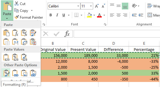
Now the next step is to apply the rules to the other rows. Copy cells A2 to E2 and select cells A3 to E6. From the Paste Special dialog box select Formats or from the Paste Special menu select Formatting as shown below.
That is it for that example. There are lots of different conditional formats that are included straight out of the box so to speak. You can even partially fill a cell with colour based on its value (a bar chart within a cell). Have a play around with Conditional Formatting and bring your workbooks to life.
Conditional functions
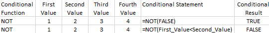
Now we will move onto formulas using conditional functions to change the values in a cell. Firstly, there are built in values for TRUE and FALSE and we will use these throughout the examples in the rest of this article. There is one function called NOT that evaluates the opposite so =NOT(TRUE) would result in FALSE. You can also evaluate formula so =NOT(1=2) would give you the opposite of false which is TRUE. You can see a couple of examples below.
All of the screenshots below use the same first, second, third and fourth values as the screenshot above so I haven’t repeated that in my screen capture. By the way, if you are wondering I use Snag-it. Towards the end of the article, where I haven’t used the same values 1, 2, 3 and 4 then I’ve captured those areas as well. All of the examples used here, including the conditional formatting can be downloaded here ExcelConditions.xlsx.
Now onto my most used conditional statement, IF. The syntax of the IF statement is IF(conditional_statement,true_value,false_value) representing if this conditional statement is true show this true value otherwise show the false value.
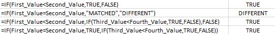
In my examples, I have first used =IF(First_Value<Second_Value,TRUE,FALSE) and this returns TRUE as the condition 1 is less than 2. In the second IF example, I have replaced the conditional statement to provide a negative result but I’ve also shown that the true and false values do not have to be TRUE or FALSE but using some text. =IF(First_Value=Second_Value,”MATCHED”,”DIFFERENT”) and this returns the text DIFFERENT as the condition 1 equals 2 is not true.
The screenshot below shows two more examples of what you can do with the true and false values, you can substitute these for other conditional statements and this is called nesting. In the first I am only returning a true value if both conditions are met. As 1 is less than 2 and 3 is less than 4, it results in TRUE being returned. In the final nested IF statement, I am returning TRUE is either of the conditions have been met.
The first of those nested IF statements where both conditions have to be met to return TRUE can be simplified using an AND statement and the second where either condition is true can be simplified using an OR statement. We will cover both of those now.
The AND statement follows this syntax; AND(conditional_statement_1, conditional_statement_2, conditional_statement_3 and so on). Each conditional statement is separated by a comma. The OR statement has exactly the same syntax except you use the OR function rather than AND.
In the AND statement all conditions are evaluated and if all are true they return TRUE.
In the OR statement if any of the evaluated conditions are true, it returns TRUE. Unlike the AND statement if the OR statement finds a suitable true condition it stops evaluating other conditions and returns TRUE. So on to some examples.
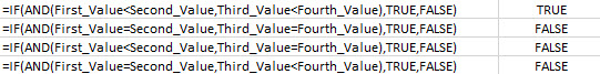
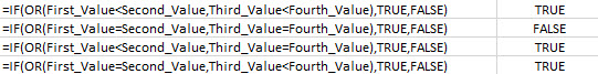
=IF(AND(First_Value<Second_Value,Third_Value<Fourth_Value),TRUE,FALSE) returns TRUE because 1 is less than 2 and 3 is less than 4. However, the remaining AND examples all have at least one condition that is untrue so they return FALSE.
=IF(OR(First_Value=Second_Value,Third_Value=Fourth_Value),TRUE,FALSE) returns FALSE because neither of the two conditional statements produce a true result 1=2 and 3=4 are both negative statements. However, all of the remaining OR examples return TRUE because at least one condition is positive.
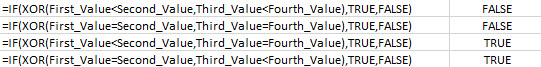
There is another type of conditional statement similar to OR that evaluates slightly differently. That is the exclusive or, XOR. Like AND, this statement evaluates all conditions but will only return TRUE if one and exactly one statement matches. So unlike OR, which will return TRUE regardless of any further positive conditions, this will only return true if it finds a positive but there are no more positives to be found.
=IF(XOR(First_Value<Second_Value,Third_Value<Fourth_Value),TRUE,FALSE) returns FALSE even though 1 is less than 2 because the second condition, 3 is less than 4, is also correct. I’ve used exactly the same statements as in the previous OR example but replaced OR with XOR.
There are two more conditional functions that I want to cover and they help you to deal with errors. They are IFERROR for if there is an error and IFNA for when something is not applicable.
Let us start with IFERROR. You can see that I have a divide by zero error in the screenshot below. This would normally have a flag next to the cell but I have told it to ignore the error.

The first row evaluates correctly with 0.5 being returned for the formula 1 divided by 2. The second row uses 1 divided by 0 and that gives a “#DIV/0!” error. The third row has the same equation but is wrapped by the IFERROR function which returns a text value, “Error”. The last row has the same values as the first but includes the IFERROR function to show that the error message text is ignored as the formula in the cell evaluates correctly.
To get a not applicable result, I’ve used the HLOOKUP function mentioned in a prior article to look for a value. I have set the approximate match to false so that rather than return something close to a value not found, it will return the Not Applicable “#N/A” result. So the first row looks for Pears in the range of Apples, Bananas, Oranges and Pears and returns Pears as it has been found. The same thing looking for Peaches does not find it so returns “#N/A” usually with an error indicator next to the cell but I told Excel to ignore it.
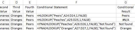
In the third and fourth rows I have wrapped the same formula in the IFNA function so that if it doesn’t find an exact match, it will not produce the Not Applicable error result but will just use some text, which I’ve set to Not Found. So now looking for Peaches returns Not found but searching for Oranges returns Oranges as it should it will only produce Not found if there wasn’t an exact match.
Finally
If you would like to have a play with the examples then you can download them here Excel Example Conditions. The first sheet in the workbook is for conditional formatting and the second sheet is for the conditional functions.
I hope you find this article and these examples useful. My previous articles on Microsoft Excel have covered, using cell reference names and named ranges, using dates and date functions, manipulating and formatting text using functions and finding a value in a range using functions.