

Everyone who uses Excel and that has written a formula (you might think that must be everyone but there are some people who just use Excel for sorting rows of data) will have used the row and column reference at some point (i.e. A1 or R1C1) or a cell range (A1:C2 or R1C1:R3C2). Anyone that has gone back to their workbook after a long time to make modifications or anyone that has to modify or decipher someone else’s workbook will curse those row and column references.
So what can you do about it? Using the naming feature within Excel you can make your life (and those of reviewers) a lot easier. It is very easy to do and I’ll show you how to name individual cells or a range of cells such as a table of data and then how to use these names in formula.
You can name a cell or range of cells in three ways:
- Using the Name Box to enter a name
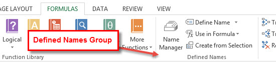
- Using the Defined Names group on the Formula tab by clicking Create From Selection
- Using the Defined Names group on the Formula tab by clicking Name Manager or Define Name
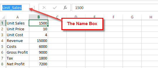
The first example is to do with naming cells and using them in formula. In this example, I have a simple product sales report showing the number of units sold and working out the net profit.
Cell B1 contains the Unit Sales, B2 the Unit Price and B3 the Unit Cost. These are inputs and are used within the formula contained in B4 onwards. The formula in B4, Revenue, is =B1*B2 and in B5, Costs, it is =B1*B3. Gross Profit, B6, is calculated using the results of B4 minus B5, =B4-B5. B7, Tax, is 20% of B6, =B6*0.2 and finally, B8, shows the Net Profit, B6 minus B7, =B6-B7.
I could easily rewrite this in a much less confusing way to say that Unit Sales x Unit Price = Revenue, Unit Sales x Unit Cost = Costs, Revenue – Costs = Gross Profit, 20% of Gross Profit = Tax and Gross Profit – Tax = Net Profit. Much simpler to read using names rather than cell references.
For each cell in Column B, you need to give it a name. As names cannot contain spaces, I’ve used the names as from Column A replacing the space with an underscore so Unit Sales becomes Unit_Sales. You can go through each individually using the Name Box.
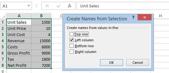
Or you can highlight the whole lot, all cells in A and B and use the Create From Selection tool. This tool replaces any spaces with the underscore character automatically.
Neither method actually goes through your formula and replaces the formula so you can either do that manually or if you have a very complex worksheet then you might want to use Find & Replace (in Formulas) by entering each new Find (i.e. B1) and Replace (i.e. Unit_Sales). The formula then become much easier to read. If you are doing this manually, then to save typing mistakes, you might want to use the Use in Formula tool within the Defined Names group.
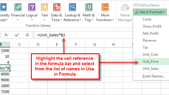
So now Revenue equals =Unit_Sales*Unit_Price, Costs are =Unit_Sales*Unit_Cost, Gross Profit is =Revenue-Costs, Tax will be =Gross_Profit*0.2 and Net Profit is =Gross_Profit-Tax.
Much easier to read. Now how about using a named range. I’ll continue with the same example but let’s say that the tax rate is calculated by Revenue in bands. Firstly I define my table with the minimum amount needed to qualify for that rate and the rate itself in the next column (I’ve used column D and E on the same worksheet but these could be on a different worksheet). This table is going to be used in a VLOOKUP function so it needs to be sorted into order and I’ll use the default functionality so I don’t have to get an exact match but it will return the closest matching value lower than it.
To name the range, just highlight the table (if you’ve used column headers make sure you exclude those) and type the name in the Name Box. In this example, I’ve called it Tax_Table.
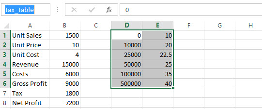
Now all I need to do is replace the Tax calculation in B7 with =Gross_Profit*(VLOOKUP(Revenue,Tax_Table,2)/100). The default action for VLOOKUP is to go through a table from top to bottom and search within the first column for a matching value. When it finds something that is greater than that value, it returns the previous matched value so in my case it matches 0 and 10,000 as these are both below 15,000 but it does not match 25,000 so it returns its last best match and that was the value used for 10,000. The 2 in the VLOOKUP function tells it to return the value from the second column in the table. You can also add an optional parameter to VLOOKUP and if you set that to FALSE it will return a value only if it finds an exact match otherwise it will return an error. We don’t want that functionality as we would have to specify a tax rate for all possible values in our range. Lastly, I never defined the rates as percentages so the VLOOKUP result needs to be divided by 100 as well.
Finally, in this article, I just want to cover the Name Manager. You can get to it from the Defined Names group and as its name might suggest, this is where you can add, edit or delete all the names defined in your workbook. Particularly useful, if you make a mistake when entering a name.
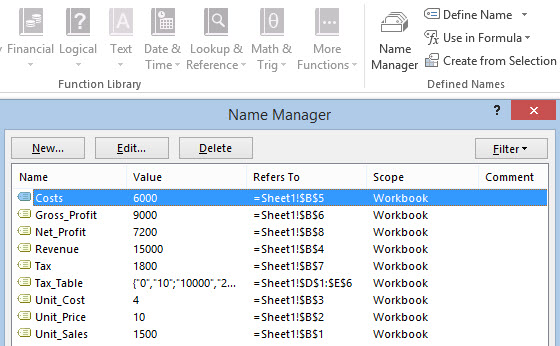
You can use the Name Manager filter to help you find things like names that have errors in your workbook.
I hope that you agree that using cell references and named ranges makes it a whole lot easier for anyone peer reviewing your work or for you to pick again in the future. If you haven’t already started using names for everything in your workbook then you should do so from now on and if you know anyone else that you think could benefit please share this with them.
If you want to download the example used here then click the link here ExcelNamedRange.xlsx.