

Following on from my other Microsoft Excel articles, this one is devoted to looking up information from within a range of values such as a table of data but using the functions that Excel provides.
We will look at four functions used for finding operations within Excel; VLOOKUP, HLOOKUP, MATCH and INDEX. First we will have an explanation of each and then walk through some examples of their usage. Finally in this article I will explain how to look up a value in a table based on multiple criteria using SUMPRODUCT.
Excel finding function descriptions
INDEX(array of values, row number, column number)
The INDEX function allows you to find a value within an array of values (usually a table). It takes three arguments (an argument is a value, a range or could even be another formula). The array of values (i.e. the range which can be a single row or column or have multiple rows and columns such as a table), the row and column number for which to return the intersecting value. To put it simply, specifying INDEX(my_table,3,4) will return the value of the fourth column on the third row.
You can also replace either row number of column number with a zero to specify that it should use all values of the row or column, in which case it will return an array of values rather than a single value. For example INDEX(my_table,0,4) returns all values of column 4 in my table.
MATCH(value to find, array of values, [match type])
The MATCH function finds the first occurrence of a value to find within an array of values. The function returns an error if not found or the position in the sequence of the first occurrence. The match type is optional so it can be left out or can be specified with 0, 1 or -1. Leaving it out assumes 0 as the default match type. The 0 is for an exact match but if no exact match is found you can tell Excel what do return in its place with 1 being the value nearest but below the value specified and -1 being the value higher than the one specified. However, any match type other than 0 only works when the array of values are in ascending order.
VLOOKUP(value to find, table of values, column number, [range lookup])
The VLOOKUP function stands for Vertical Lookup and searches through the rows of the first column in a table of values and returns the value from a column number specified.
The values in the first column must be in ascending order from top to bottom. If you have a table of values and you want to find a record by using the identifier in the first column and return a value from the row of date for that identifier then this is a very useful function. The range lookup is an optional setting with TRUE being a nearest match and FALSE being an exact match. FALSE will return an error if not found whereas TRUE will return the exact match if it is found but if not will still return the value in the sequence at the position before the value to find.
For example a search for “Spurs” in the following data sequence; “Queens Park Rangers”, “Southampton”, “Stoke City”, “Sunderland”, “Swansea City”, “Tottenham Hotspur” and “West Bromwich Albion” would produce “#N/A” if the range lookup was FALSE and “Southampton” if the range lookup was TRUE.
HLOOKUP(value to find, array of values, row number, [range lookup])
The HLOOKUP function stands for Horizontal Lookup and searches through the columns of the first row in an array of values and returns the value from a row number specified. The values in the first row must be in ascending order from left to right. Other than that it works and behaves in exactly the same was as a VLOOKUP.
MATCH and INDEX work fine on a range that has more than one column and row but VLOOKUP and HLOOKUP require a table with more than one column and row.
Excel finding function example workbook
The following examples look at the fixture list at the start of the English Premier League football season. I will work though a few situations where you can combine them to get the data you require.
If you want to download these examples you can do so here Fixtures.xlsx. The workbook has 3 sheets; Matches, MatchDays and Calculations.
At the beginning of the season, the fixtures are set on a week commencing basis for all 38 games and then the TV companies as well as UAFA rules come in to place and quite a few of the games are moved to alternative days. During the season, games are also postponed to other days but this workbook was put together early in August before the season started so we will just use the Match Week Number and the Date of the Commencement of fixtures for that week.
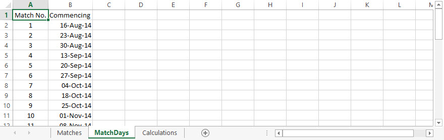
MatchDays has a simple table with two columns depicting Week Number and Date Commencing.
The Matches sheet contains a table that has its first column for the home team and first row for the away team names. So basically, using the rows and columns you can look up a home team and an away team and at their intersection find the week number when the game is due to be played. We can then look up the week commencing date on the MatchDays sheet.
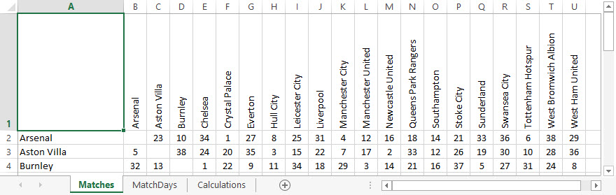
In the workbook, I’ve used some named ranges. On the MatchDays sheet the only one is Match_Days for the area of the table. On the Matches sheet, the named ranges are Matches_Matrix for the whole of the table, Match_Home_Teams for the home team column of team names and Match_Away_Teams for the away team row of team names. There are also named ranges for each home team using that teams name for some of the later examples. If you want a reminder about specifying named ranges please visit my page “Using Excel cell references and named ranges“.
Finding information examples
In the first examples, I will do something straight forward to show the functionality of the INDEX and MATCH functions.
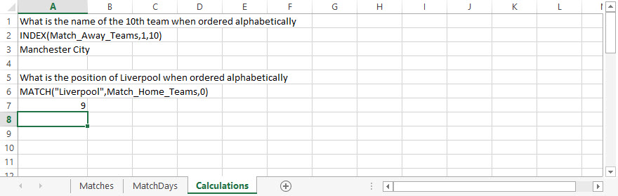
You can use the INDEX function to return a value from a list at a specified position. So if I were to ask, “What is the name of the 10th team when ordered alphabetically” I would use INDEX(Match_Away_Teams,1,10) to show that the 10th team is Manchester City.
We can also determine the position within a range of values of that a value occurs by using MATCH. So if you were to ask, “What is the position of Liverpool when the teams are ordered alphabetically” I would use MATCH(“Liverpool”,Match_Home_Teams,0) to show that the position is 9th.
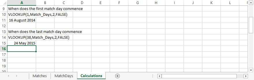
Now let us find some dates based on the MatchDays table using VLOOKUP. The table is in ascending order and I know there is a value for the commencement week for each week from 1 to 38 so I can use VLOOKUP(1,Match_Days,2,FALSE) to show the first match day (week 1) commences on the 16th August 2014 (column 2) and that the last match day (week 38) is on the 24th May 2015 using VLOOKUP(38,Match_Days,2,FALSE).
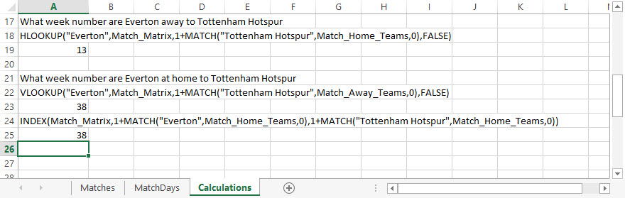
Now on to something more interesting. I’m going to use a combination of methods to look up when two teams play each other. Firstly, what week number are Everton away to Tottenham Hotspur and then what week number does the corresponding home fixture commence.
I can see that using HLOOKUP(“Everton”,Match_Matrix,1+MATCH(“Tottenham Hostpur”,Match_Home_Teams,0),FALSE) shows that Everton are away to Tottenham on the 13th week. What I am doing here is using a horizontal lookup for the column of “Everton” on the Match_Matrix table and looking up the row number using the MATCH function on the Match_Home_Team but I have to add 1 to the returned value because the Match_Matrix has both its first row and column with team names and not the matches themselves.
The corresponding fixture to find when Everton are at home to Tottenham could have been accomplished using the previous code but swapping the team names around or we can use the VLOOKUP with the same values. As a MATCH on Match_Away_Teams and Match_Home_Teams would return the same value I didn’t really need to change that in the syntax but I did do so.
There is a slightly longer way of performing the same functionality without VLOOKUP or HLOOKUP and that is using INDEX. INDEX(Match_Matrix,1+MATCH(“Everton”,Match_Home_Teams,0),1+MATCH(“Tottenham Hotspur”,Match_Home_Teams,0)) will also show that Everton are at home to Tottenham on week 38. The INDEX function uses the same table but within it you specify the row and column.
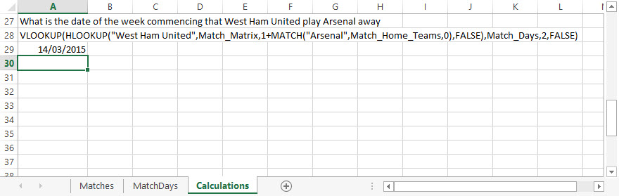
This next example gets the actual date by using a VLOOKUP on Match_Days for the week returned from a HLOOKUP of when West Ham are away to Arsenal. The result of 14 th March 2015 is given for as a result for VLOOKUP(HLOOKUP(“West Ham United”,Match_Matrix,1+MATCH(“Arsenal”,Match_Home_Teams,0),FALSE),Match_Days,2,FALSE).
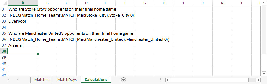
Now let us say that we want to find out who a team is playing on a particular week number. For these examples I’ve simplified the code by introducing a named range for each home team’s fixture weeks. So Newcastle United have a named range of Newcastle_United.
Let’s find out who Stoke City are playing on the first game of the season. This can be done using INDEX(Match_Home_Teams,MATCH(Max(Stoke_City),Stoke_City,0)) to return Liverpool as Stoke’s opponents.
I have not only introduced the additional named range for each team but I’ve also used the MAX function which takes a range of values and returns the highest regardless of the order. Basically, because a team could be home or away on the last day of the season I have used the MAX function to determine the week number of their final home game. For stoke they are at home on week 38 but in my next example, who are Manchester Unit playing on their last home match, I find that their last home game is in week 37 against Arsenal.
Using multiple criteria within Excel to find a value
We have covered the different ways to quickly find something from within something in Excel using INDEX, MATCH, VLOOKUP and HLOOKUP. All of these functions have something in common and that is they all find a single value within a table or array of values.
If you want to find values based on multiple criteria it gets a bit more complex and that job is usually undertaken by a database. However, Excel does have a function that can be used and it is called SUMPRODUCT. I had better warn you that it is not very fast when you have a lot of data but you can specify any number of criteria to look up on a table. You can download the following example here sumproduct.xlsx.
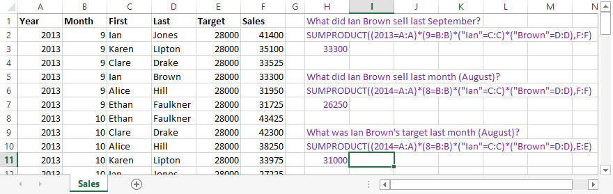
In this example, I’ve set up a table for sales and it does not need to be in any particular order as SUMPRODUCT will search through until it finds a match for the criteria you specify. The syntax to use is SUMPRODUCT(criteria, array of results). So for my example, let’s say I want to find what Ian Brown’s sales were in August 2014. I would write SUMPRODUCT((2014=A:A)*(8=B:B)*(“Ian”=C:C)*(“Brown”=D:D),F:F). Each of the criteria you specify you wrap in parentheses and use the multiplication operator to join them. I haven’t named any ranges here but you can see that I am saying column A must have 2014 in it, column B must have an 8 in it, column C must have the value “Ian” and column D must equal “Brown”. The final part is what to return and I want the corresponding value from the Sales column, which is column F.
That’s it for finding values using functions in Excel and I hope you found these examples useful.