

In this article, I broadly cover Microsoft Excel’s Paste Special functions with an example using the Operations of Paste Special.
Before we get to an example some background is needed. Each cell in Microsoft Excel is made up of three parts; values (data), formula and format. Copying and pasting from one cell (or range of cells) to another copies all three exactly as they are. The formula remains the same (but relative to the new cell position), the values/data remains the same (unless it is formula driven) and the format remains unchanged (unless it is conditional on the data).
The cell (or cell range) does not need to be copied exactly and there are several options to help you achieve that on the “paste options” context menu or through the “paste special” dialog box. These help you to manipulate the result when using the pasting feature. It is quite often quicker than using a formula or other methods to achieve the same result. I covered the “transpose” paste option in a previous article to show how to convert a cell range from columns to rows or vice-versa, so I won’t cover that here.
Example spreadsheet
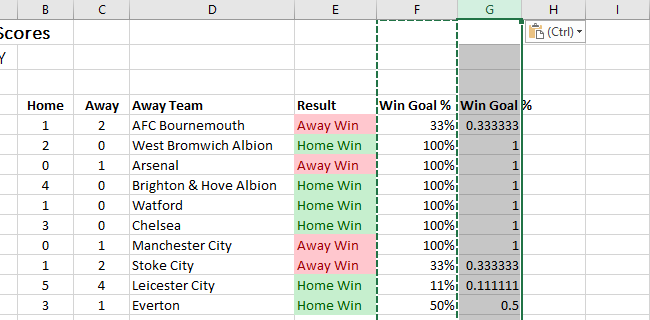
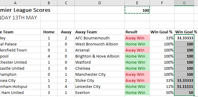
First, I will use an example spreadsheet (which you can download 20180513-Scores if you would like). It shows the English Premier League football scores for the last day of the 2017/2018 season, which concluded today. I have some basic formatting and a couple of columns with formula in them, one of which has conditional formatting.
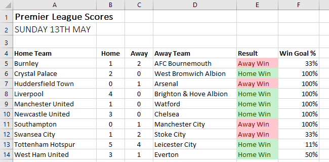
Column E shows the outcome of the match, either a draw or whether the home or away team won. It has conditional formatting for green for home, red for away and yellow for a draw. The final column shows how many goals the winner scored out of the total number of goals which is 50% for a score draw and 0% for a non-scoring draw. A completely meaningless column but has a percentage in it that I will use in this article.
Copy and Paste
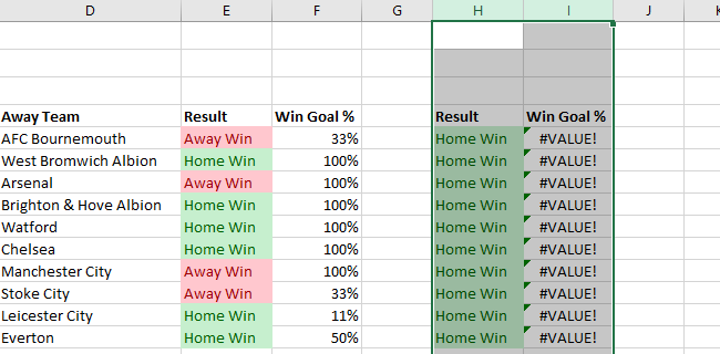
First of all, if I copy (Ctrl+C) and paste (Ctrl+V) these cells anywhere else they will paste any data, any formula and any formatting to the new location and will maintain relativity. What that means is that if I copy columns A-F to columns H-M then everything will copy and the formula will show the correct result based on the scores in the new location. If you tried that, undo it. However, if I copy just the formula columns E-F to H-I then they will be evaluated based on the wrong location. If you compare the formula in E5 with H5 you will see that F5 is not evaluation the scores in columns B and C.
E5: =IF(B5=C5,”Draw”,IF(B5<C5,”Away Win”,”Home Win”))
H5: =IF(E5=F5,”Draw”,IF(E5<F5,”Away Win”,”Home Win”))
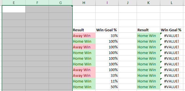
If I had used cell names then the values would be correct. However, knowing that the cell references remain relational can also be useful. If I really did want the formula to resolve correctly and I wanted to keep it in both E5 and H5 for example, I could copy as above which keeps the correct formula relationship but wrong values.
Then insert three columns (which doesn’t affect formula), copy back my originals (now in columns K and L) to empty columns E and F â then delete columns K and L.
Anyway, that is nothing to do with Paste Special, other than to show one of the issues that can be encountered when pasting formula. If you have been following above, and want to continue following then delete all of those extra columns.
Paste Options
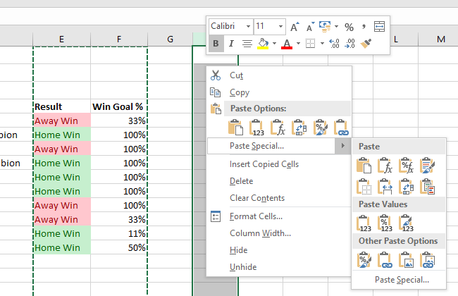
First of all to get the paste options context menu showing you have to copy (Ctrl+C). Normally, you would either paste (Ctrl+V) or get the paste special dialog box up (Ctrl+Alt+V). To get the context menu for the popular paste options up (quick short cuts), you have to right click on your destination cell(s). You will see a “paste options” section where the most common options are shown from left to right; Paste, Values (data only), Formulas, Transpose, Formats and Paste Link (just references to the original cell).
Beneath these you will see Paste Special which is used to bring up the dialog box where you can perform any of these and a lot more. To the right of Paste Special is an expansion marker that if you move your mouse over brings up some more popular options including some combinations. Some are already mentioned but there are Formulas & Numbering Format, No Borders, Keep Column Widths, Merge Conditional Formatting, Values & Number Formatting, Values & Source Formatting, Picture and Linked Picture.
These are quick shortcuts to behaviours that you can achieve using the Paste Special dialog box. For example, if you want to Paste Values you can use the icon with 123 on a clipboard or use Values in the Paste Special dialog box.
The paste options are all straight forward and there are lots of examples everywhere. As you mouse over the popular option icons on the context menu you can see a preview of the change on the cells you intending to paste to. Also, if you make a mistake on your option, you can always repeat with another option or use the undo function.
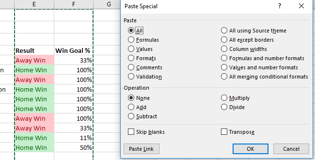
Paste Special Operations
There is one thing in the Paste Special dialog box that you might want to use that is not obvious and that is the Operations. From here you can take a mathematical action and apply it to a numeric range as a paste operation.
To see that in action follow these steps.
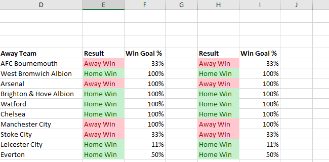
Copy column F to G but only paste values. You can see that the percentages are not showing correctly in column G as they are the values of the percentages.
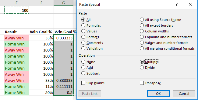
We could format the column or could have pasted values and number formats but let us use a multiply operation (after all the header shows a % symbol anyway).
The first thing to do is indicate a value on the spreadsheet to multiply by. For this example, I added 100 to cell E1.
Then copy the cell E1, go to the range to apply the paste option operation to (G5:G14) and click Ctrl+Alt+V then select M or click Multiply and OK.
Obviously, this was just a simple example and there are other ways to do the same thing. For example, using formula in another column you could paste the values back over the top. Using the paste special operations is a little quicker than writing formula, pasting values and deleting the formula.
One thing to be wary of is that the paste special operations are applied to all cells in a range by default. If you selected the column rather than the cell range, all non-blank cells in the column will have a value of zero. This is because the default value for an empty cell is zero and multiplying that by 100 is 0. If you have selected the whole column you can avoid it filling the empty cells by checking the box “Skip blanks” within the Paste Special dialog box.