

A while back we had a situation where we had collected a set of information from various sources and wanted to get all of it into the same Excel Worksheet and I was asked if I could help. There were about 60 spreadsheets all with the same columns but with a variable number of rows and of course, different data. The requester had linked all 60-odd spreadsheets to a master Workbook and wanted to know how to get the information from each transferred to a single master sheet that he could share as a consolidated list. This process needed to be repeatable as the authors of the 60-odd different worksheets would update these regularly and he wanted to the master sheet to always have the latest information with minimal effort.
I showed him what to do using the data manipulation features of Excel 2016. In this article, I will walk through those steps using some made up information rather than what he was consolidating.
Example Set Up
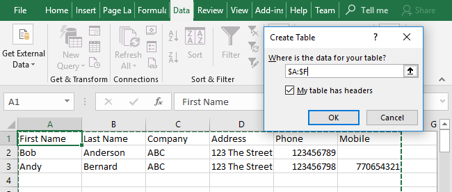
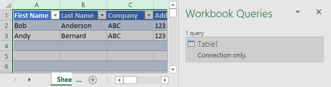
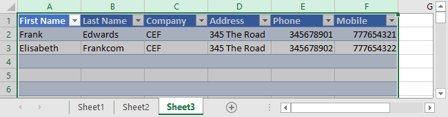
For simplicity, I will not link each sheet to a source sheet as that is simple to do but instead have created 3 sheets each with some dummy information and put these in the same workbook. In the real world, the authors would not have access to the master workbook so they would edit their own data sheet which this workbook pulls in. As I don’t want to disclose the information he was consolidating, I will just use dummy contact details as shown below.
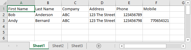
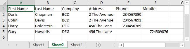
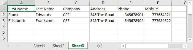
I could have prepared this data into tables beforehand but it is not required as the following steps will convert the data range into tables. So, just for clarity, I have 3 sheets of contact details that I want to include in a dynamic master sheet. These contact details can change and if they do, I want to be able to refresh the master sheet rather than recreate it.
First we need to establish a data connection from the “Data” tab on the Excel ribbon, “From Table” in the “Get & Transform” section, as if these were tables.
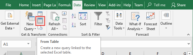
However, do not accept the range proposed by the dialog box asking where your data-table is, select all rows instead. When in that dialog box formula range, go to your sheet and starting from the first column drag the range to the last column including all rows so that in future newly added data will be included. Make sure you have a check mark in the headers (assuming you have column headers).
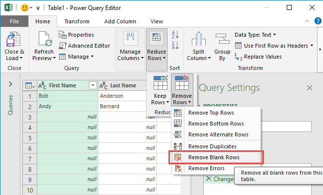
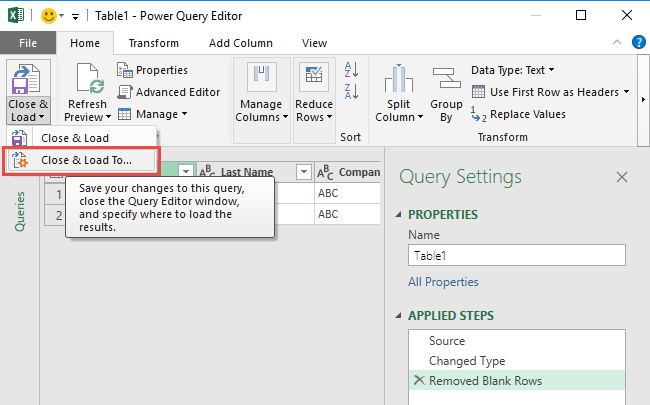
The Power Query Editor will show but but we don’t want to include rows that are empty. Select “Remove Blank Rows” from the menu under “Reduce Rows” – “Remove Rows”. Then under the “Close & Load” menu select “Close & Load To”.
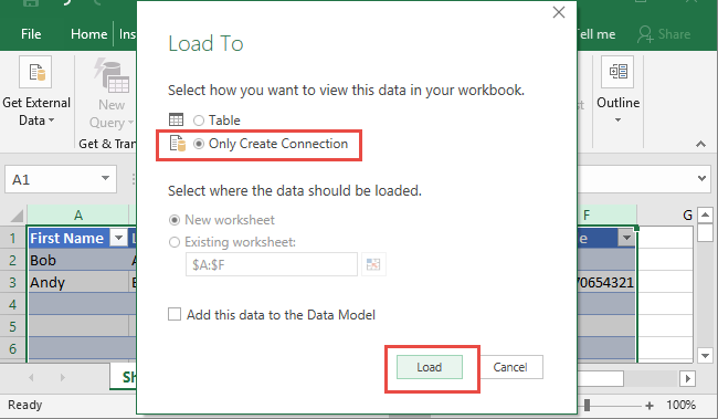
When prompted select “Only Load Connection” and click the “Load” button.
You will then see the Connections section opened up.
Repeat the steps above for the other sheets so you have all the connections to each sheet that remove blank rows.
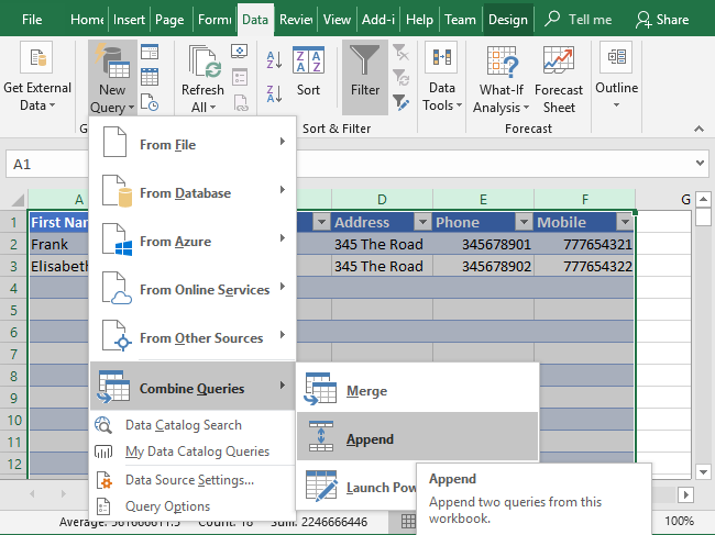
Now for the summary sheet, where the magic happens, we need another query this time select an “Append” from the “Combine Queries” found on the “New Query” menu in the “Get & Transform” section of the “Data” tab. We are using Append because we are collating all rows of data, there are other options for different types of data joining.
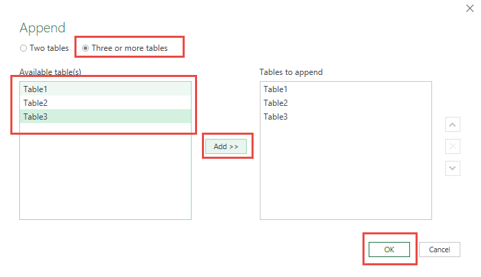
Select 3 or more when prompted.
Then add the table query connections you created earlier by selecting them and clicking “Add”. When they are all showing on the right-hand panel, click “OK”.
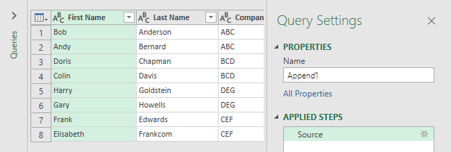
You will then see a preview of the data that will be included on the master sheet.
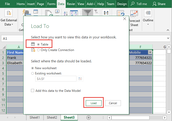
This time when we close, we will load it to a destination sheet. As before “Close and Load To”. Then leave as the default, Table and New worksheet. Then click Load.
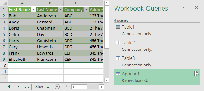
You will see a new sheet created with your data. The Workbook Queries window will also be displayed with the new query name.
Now when you add a row or change your data whenever you like and you can refresh that new Append query (or from anywhere on the master table).
Let’s do that.
Refreshing data
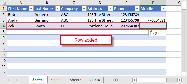
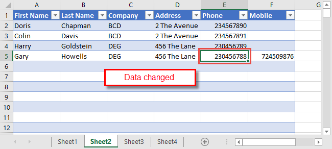
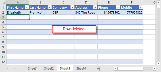
First I will make some changes to each sheet, I’ve added a new row of data on one, altered a row of data on another by adding a phone number and deleted a row of data on the last.
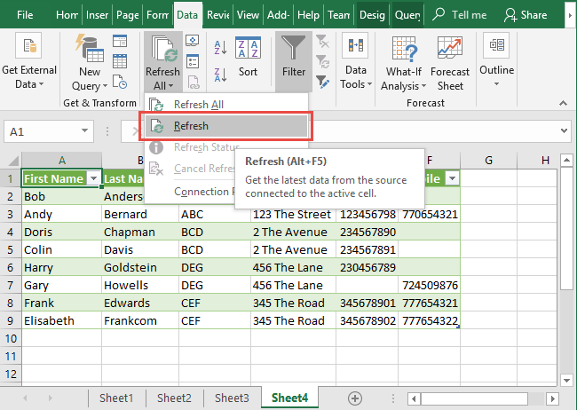
After all the adjustments have been made you can refresh all of the queries to feed your adjustments into the master sheet.
From anywhere you can go to the Data tab, select “Refresh All” from the “Refresh All” menu. Alternatively, if you only want to refresh the summary you can go to the summary table and select “Refresh” from the same menu or press Alt+F5 on a Windows keyboard.
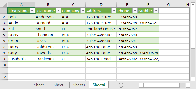
You can see that the data for Gary Howells has been changed, Frank Edwards deleted and Zak Smith added.
Examples Workbooks
I’ve included the workbook at it was at the start and the other as it was when finished. If you want to see the final outcome you can have a look at Excel Data Consolidation Finished Example, “Finished.xlsx“, but if you want to walk through this article step by step then you can use “Start.xlxs“.